Code
# code to generate dataset

rm(list=ls())

# Set seed for reproducibility
set.seed(123)

# Generate sample data
data <- rbind(
  matrix(rnorm(100, mean = 0.5), ncol = 2),
  matrix(rnorm(100, mean = 3), ncol = 2)
)As we learned earlier in the module, clustering involves grouping a set of objects in such a way that objects in the same group, or cluster, are more similar to each other than to those in other clusters.
This is fundamental in discovering the inherent groupings within our data. It provides information about its structure without the need for predefined categories or labels.
Clustering algorithms organise data into meaningful or useful groups, where the degree of association within-groups is maximised and between-groups is minimised.
Clustering methods can be categorised into several types:
partitioning methods
hierarchical methods
density-based methods (not covered in this module)
grid-based methods (not covered in this module)
The objective of K-Means Clustering is to partition \(n\) observations into \(k\) clusters, in which each observation belongs to the cluster with the nearest mean.
This is done by an algorithm that:
initialises k centroids randomly.
assigns each point to the closest centroid, forming k clusters.
recalculates the centroids as the mean of all points in each cluster.
repeats steps 2 and 3 until convergence.
To demonstrate a simple example of using k-means clustering in R, I’ll create a small dataset with two variables, and apply the kmeans function.
Remember, this is unsupervised learning because we aren’t telling the model how to group the observations.
# code to generate dataset
rm(list=ls())
# Set seed for reproducibility
set.seed(123)
# Generate sample data
data <- rbind(
matrix(rnorm(100, mean = 0.5), ncol = 2),
matrix(rnorm(100, mean = 3), ncol = 2)
)A raw plot of the data doesn’t reveal any obvious clusters in our data:
# Plot data
plot(data, col = "blue", main = "Raw Data", xlab = "Feature 1", ylab = "Feature 2", pch = 20)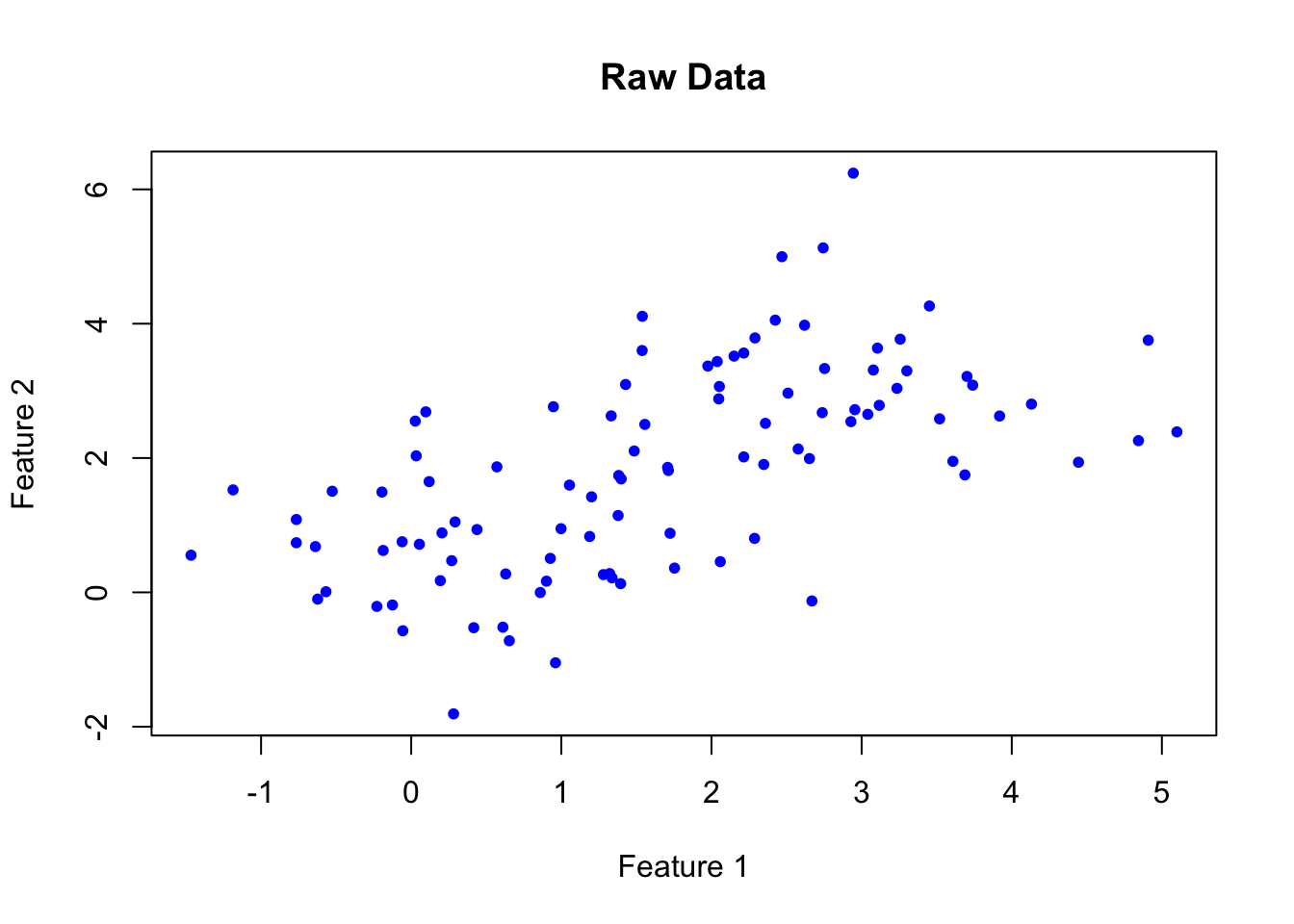
Now, we can conduct a k-means cluster analysis to divide the data into two clusters (see below for information on how we determine the optimum number of clusters).
# Apply k-means with k = 2
set.seed(123)  # Setting seed for reproducibility
kmeans_result <- kmeans(data, centers = 2)

# Plot the results
plot(data, col = kmeans_result$cluster, main = "K-Means Clustering Results", xlab = "Feature 1", ylab = "Feature 2", pch = 20)
points(kmeans_result$centers, col = 1:2, pch = 8, cex = 2)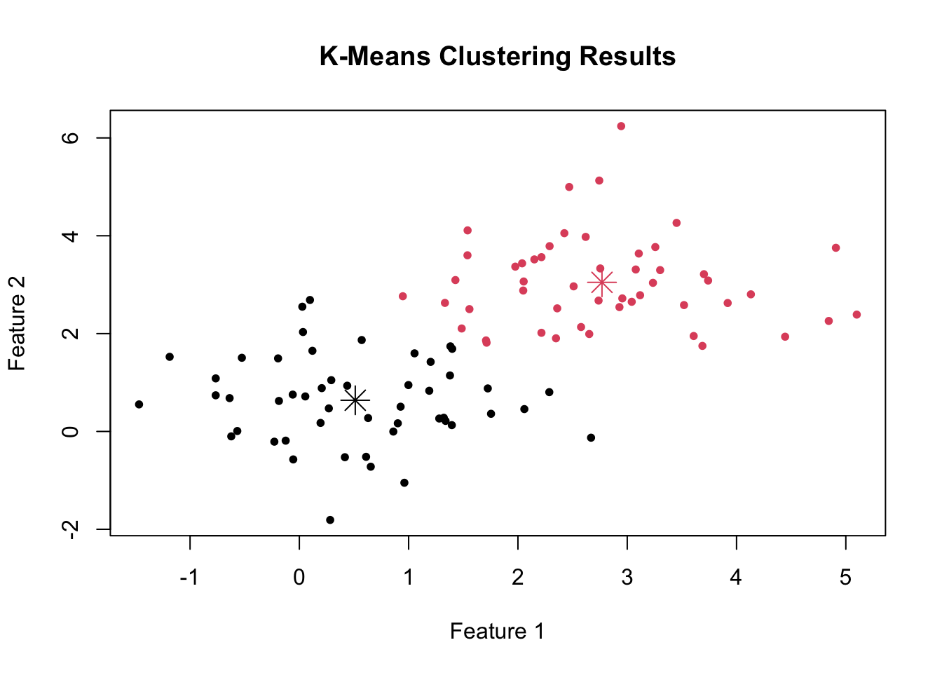
This code applies k-means clustering to the data with k = 2 and then plots the original data points colored by their assigned cluster.
The cluster centers are marked with larger symbols. You can see how k-means clustering has identified groups within the data based on their features.
Hierarchical clustering builds a hierarchy of clusters either in an agglomerative (bottom-up) or divisive (top-down) approach.
Agglomerative: Each observation starts in its own cluster, and pairs of clusters are merged as one moves up the hierarchy.
Divisive: Starts with all observations in a single cluster and iteratively splits the cluster into smaller clusters until each cluster contains only a single observation or a specified termination condition is met.
In hierarchical clustering, instead of specifying the number of clusters upfront, we build a tree of clusters and then decide how to cut the tree into clusters.
Here, we’ll use the ‘complete linkage’ method.
We’ll use the same dataset as for the k-means cluster analysis above.
# Compute the distance matrix
dist_matrix <- dist(data)

# Perform hierarchical clustering using complete linkage
hc_result <- hclust(dist_matrix, method = "complete")

# Plot the dendrogram
plot(hc_result, main = "Hierarchical Clustering Dendrogram", xlab = "Points", ylab = "Distance")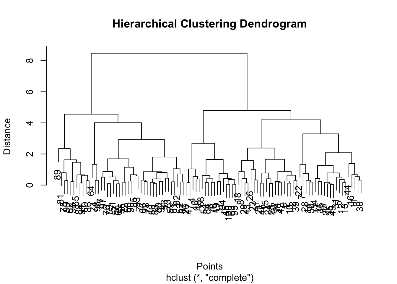
This code calculates the pairwise distances between points and then applies hierarchical clustering. The plot function then generates a dendrogram representing the hierarchical clustering result.
As can be seen from the dendrogram, the data appears to divide into two clusters. We can check our assumption using the methods below.
To cut the dendrogram into clusters, we can use the cutree function:
# Cut the tree into 2 clusters
clusters <- cutree(hc_result, k = 2)

# Plot the original data colored by clusters
plot(data, col = clusters, main = "Hierarchical Clustering Results", xlab = "Feature 1", ylab = "Feature 2", pch = 20)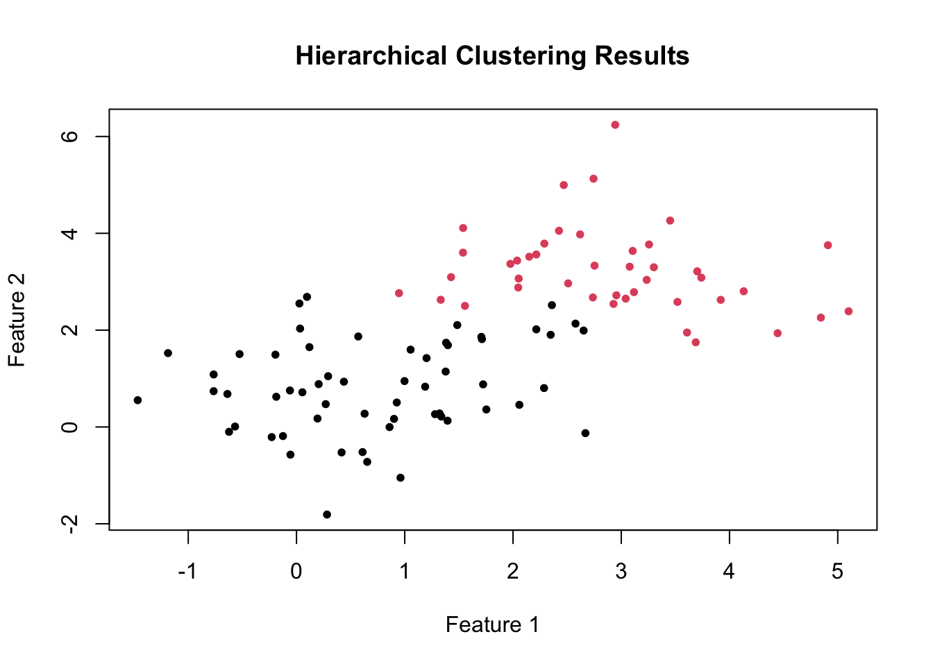
As before, this code cuts the hierarchical tree into two clusters and plots the data points colored by their cluster membership.
The cutree function is used to specify the number of clusters (k = 2) we want to extract from the hierarchical tree.
In the steps above, I decided to ask the algorithm to identify 2 clusters within the raw data. There are a number of different techniques we can use to decide what the ‘best’ number of clusters is in our data.
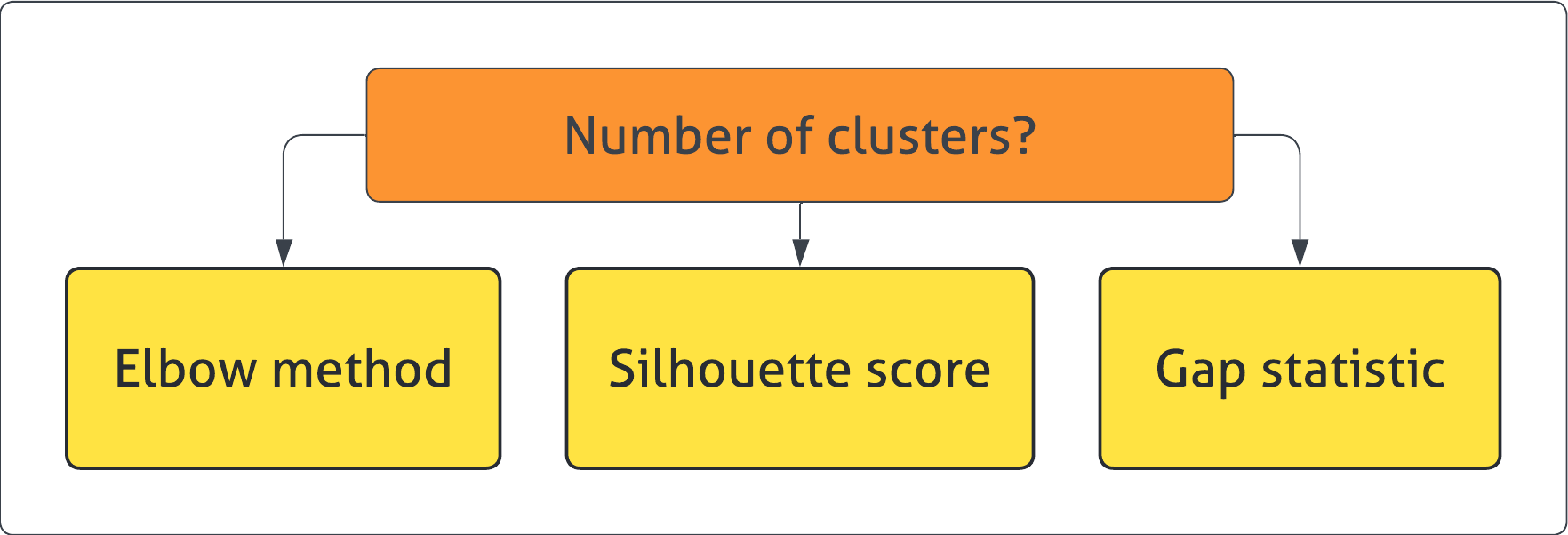
Elbow Method
This is one of the most common techniques used to determine the optimal number of clusters.
We run the k-means algorithm on the dataset for a range of k values (e.g., 1 to 10) and for each value, calculate the sum of squared errors (SSE).
The SSE tends to decrease as you increase \(k\), because the distances of the points from the centroids decrease.
We look for a “knee” in the plot of SSE versus \(k\), which resembles an elbow. The idea is that the elbow point is a good ‘trade-off’ between low SSE and simplicity of the model.
library(cluster)
set.seed(123)

wss <- (nrow(data) - 1) * sum(apply(data, 2, var))
for (i in 2:15) {
  wss[i] <- sum(kmeans(data, centers = i, nstart = 20)$withinss)
}

plot(1:15, wss, type = "b", main = "Plot of SSE", xlab = "Number of Clusters", ylab = "Within groups sum of squares")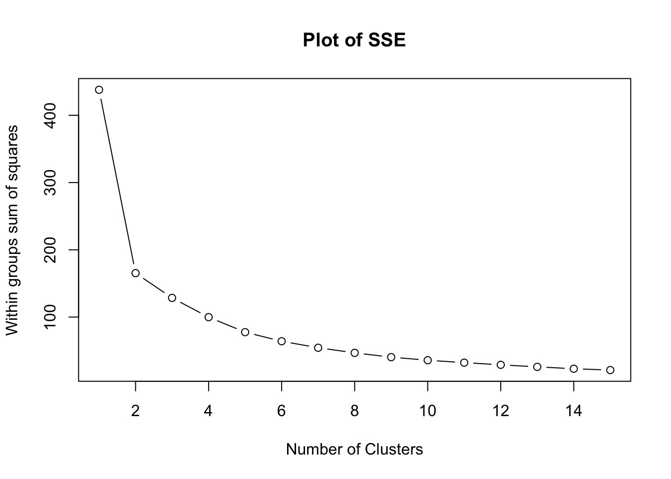
In the plot above, we can see that the ‘elbow’ appears to form after 2 clusters.
Silhouette Score
This method evaluates the consistency within clusters. For each sample, the silhouette score is a measure of how similar that point is to points in its own cluster compared to points in other clusters.
The silhouette score ranges from -1 to +1, where a high value indicates that the object is well matched to its own cluster and poorly matched to neighbouring clusters.
We can calculate the average silhouette score for different numbers of clusters and choose the number that gives the highest average score.
library(cluster)
sil_width <- numeric(15)
for (k in 2:15) {
  km.res <- kmeans(data, centers = k, nstart = 25)
  ss <- silhouette(km.res$cluster, dist(data))
  sil_width[k] <- mean(ss[, 3])
}
plot(2:15, sil_width[2:15], type = 'b', main = "Plot of Silhouette Score", xlab = "Number of Clusters", ylab = "Average Silhouette Width")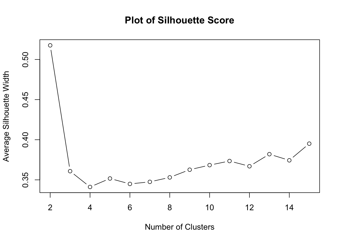
Again, note that 2 clusters produces the highest silhouette score.
Gap Statistic
Finally, the ‘gap statistic’ compares the total within intra-cluster variation for different values of k with their expected values under null reference distribution of the data.
The optimal k is the value that maximises the gap statistic, indicating that the clustering structure is far away from the random uniform distribution of points.
set.seed(123)
gap_stat <- clusGap(data, FUN = kmeans, nstart = 25, K.max = 10, B = 50)
plot(gap_stat, main = "Plot of Gap Statistic")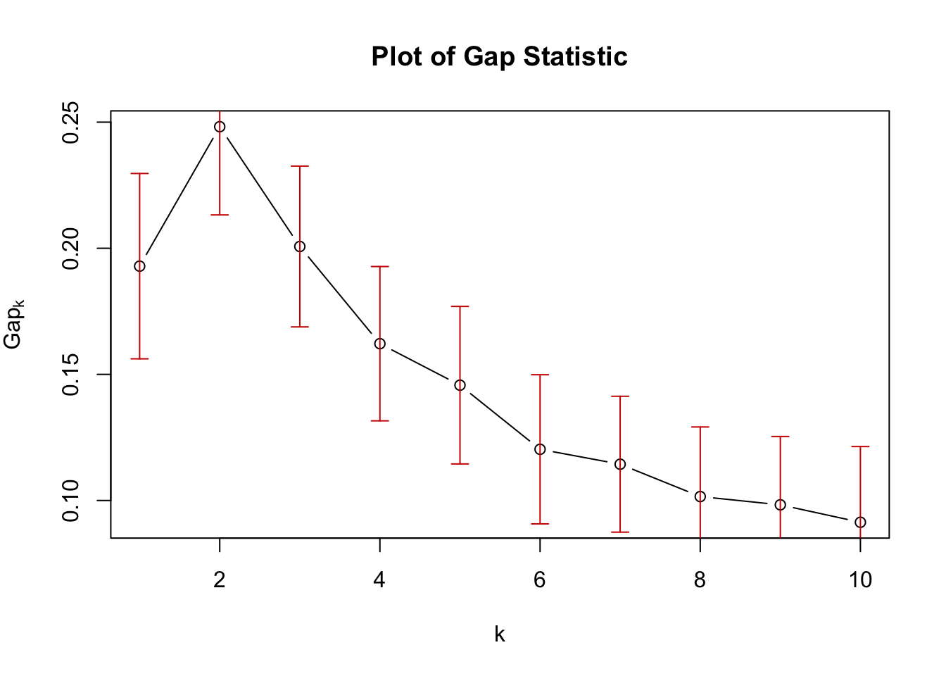
As for the other methods, 2 clusters appears to be the optimum number for our raw data.